Category Google Certification Exams

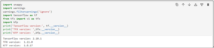
Importing packages – Pipelines using TensorFlow Extended-2

Transform:
We will create file_transform.py which will contain information about the data labels and feature engineering steps:
• Run the following mentioned code in new cells to declare variable containing file name:
TRANSFORM_MODULE_PATH = ‘file_transform.py’

• Run the following mentioned codes in a new cell to create file_transform.py file. Preprocessing (preprocessing_fn) function is where the actual alteration of the dataset occurs. It receives and returns a tensor dictionary, where tensor refers to a Tensor or SparseTensor. In our example, we are not applying any transformations, code is just mapping to the output dictionary. (%%writefile command will create the .py file with the following code in it.):
%%writefile {TRANSFORM_MODULE_PATH}
import tensorflow as tf
import tensorflow_transform as tft
NAMES = [‘AF3’,’F7’,’F3’,’FC5’,’T7’,’P7’,’O1’,’O2’,’P8’,’T8’,’FC6’,’F4’,’F8’,’AF4’]
LABEL = ‘eyeDetection’
def preprocessing_fn(raw_inputs):
processed_data = dict()
for items in NAMES:
processed_data[items]=raw_inputs[items]
processed_data[LABEL] = raw_inputs[LABEL]
return processed_data

  1. Files needs to copy into GCS bucket, run the following line of code to copy it:
    !gsutil cp file_transform.py {MODULE_FOLDER}/
  2. Run the following mentioned lines of codes in a new cell to configure transform component. Transform component is taking inputs from the example_gen and schema_gen:
    transform_data = tfx.components.Transform(
    examples=example_gen_csv.outputs[‘examples’],schema=gen_schema.outputs[‘schema’],
    module_file=os.path.join(MODULE_FOLDER, TRANSFORM_MODULE_PATH))
    context_in.run(transform_data, enable_cache=False)

Output of the transform component is as shown in Figure 8.10. Transform graph is one of the artifacts generated by the transform component and it will be used for the trainer module.

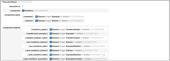
Figure 8.10: Output of transform component
Run the following mentioned codes to check few records of the transformed data (This code will not be needed during the pipeline construction):
train_sam = os.path.join(transform_data.outputs[‘transformed_examples’].get()[0].uri,’Split-train’)
filenames_tfr = [os.path.join(train_sam, name) for name in os.listdir(train_sam)]
dataset = tf.data.TFRecordDataset(filenames_tfr, compression_type=’GZIP’)

for record in dataset.take(1):
sample = tf.train.Example()
sample.ParseFromString(record.numpy())
print(sample)

Output of 1 record will be as shown in Figure 8.11:

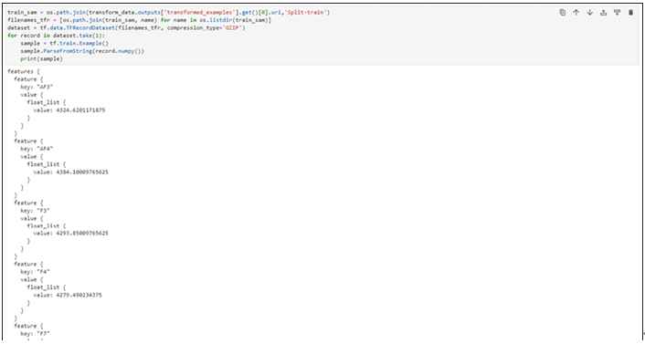
Figure 8.11: Transformed data example
Trainer:
The Trainer component is in charge of preparing the input data and training the model. It requires the ExampleGen examples, the transform, and the training code. TensorFlow Estimators, Keras models, or custom training loops can be used in the training code. When compared to other components, trainer requires more modifications in the code:
• Run the following mentioned code in the new cell, it will generate trainer.py file (Complete code is available in the repository). Trainer.py (training code) file will be the input for the trainer module. Trainer component generates two artifacts model (trained model itself) and modelrun which can be used for storing logs, this can be seen in Figure 8.12. The Trainer.py file contains four functions; high level description of those functions is:
o run_fn will be entry point to execute the training process
o _input_fn generates features and labels for training
o _get_serve_tf_examples_fn returns a function that parses a serialized tf.example
o _make_keras_model creates and returns the model for classification
%%writefile trainer.py
from typing import List
from absl import logging
import tensorflow as tf
import tensorflow_transform as tft
from tensorflow import keras
from tensorflow_transform.tf_metadata import schema_utils
from tfx import v1 as tfx
from tfx_bsl.public import tfxio
from tensorflow_metadata.proto.v0 import schema_pb2

COL_NAMES=[‘AF3’,’F7’,’F3’,’FC5’,’T7’,’P7’,’O1’,’O2’,’P8’,’T8’,’FC6’,’F4’,’F8’,’AF4’]
LABEL=”eyeDetection”
BATCH_SIZE_TRAIN = 40
BATCH_SIZE_EVAL = 20
def _input_fn(files,accessor,transform_output,size) -> tf.data.Dataset:
Creates datasets and apply transformations on them and return.
Refer the repository for code block of the function
return dataset.map(apply_transform_fn).repeat()
def _get_serve_tf_examples_fn(model, transform_output):
To parse the serialized examples and return.
Refer the repository for code block of the function
return serve_tf_examples_fn
def _make_keras_model() -> tf.keras.Model:
Create model with layers, loss functions to be used and return.
Refer the repository for code block of the function
return model_classification

def run_fn(fn_args: tfx.components.FnArgs):
tf_transform = tft.TFTransformOutput(fn_args.transform_output)
train_samples = _input_fn(_args.train_files, _args.data_accessor, tf_transform, =BATCH_SIZE_TRAIN)
eval_samples = _input_fn(_args.eval_files, _args.data_accessor, tf_transform, =BATCH_SIZE_EVAL)
model_classification = _make_keras_model()
model_classification.fit(
train_samples,
steps_per_epoch=fn_args.train_steps,
validation_data=eval_samples,
validation_steps=fn_args.eval_steps)
sign = {
“serving_default”: _get_serve_tf_examples_fn(model_classification, tf_transform),
}
model_classification.save(fn_args.serving_model_dir, save_format=’tf’,signatures=sign)

  1. Run the following code to copy the trainer.py to GCS storage:
    !gsutil cp trainer.py {MODULE_FOLDER}/
  2. Run the following code to initiate the trainer component. trainer_file=”trainer.py”:
    trainer_file_path=os.path.join(MODULE_FOLDER, trainer_file)
    model_trainer = tfx.components.Trainer(
    examples=example_gen_csv.outputs[“examples”],
    transform_graph=transform_data.outputs[“transform_graph”],
    train_args=tfx.proto.TrainArgs(num_steps=200),
    eval_args=tfx.proto.EvalArgs(num_steps=10),
    module_file=trainer_file_path,
    )
    context_in.run(model_trainer, enable_cache=False)

The output of the trainer component is as shown in the following figure:

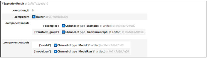
Figure 8.12: Output of the trainer component

Importing packages – Pipelines using TensorFlow Extended-1

Step 6: Importing packages
Run the following mentioned line of codes to import required packages:
import tensorflow as tf
import tensorflow_transform as tft
from tensorflow import keras
from tensorflow_transform.tf_metadata import schema_utils
from tfx import v1 as tfx
from tfx_bsl.public import tfxio
from tfx.components.base import executor_spec
from tfx.orchestration.experimental.interactive.interactive_context import InteractiveContext
from tensorflow_metadata.proto.v0 import schema_pb2
import os
from typing import List

Step 7: Understanding a few TFX components from code
Even before jumping into pipeline creation and execution, let us try to understand how a few of the TFX components can be used individually and analyze the output of those components. Let us start with the data Examplegen component.
Examplegen: Run the following code in a new cell:
context_in = InteractiveContext()
example_gen_csv = tfx.components.CsvExampleGen(input_base=INPUT_DATA_DIR)
context_in.run(example_gen_csv)

Examplegen component can read the data from various sources and data types such as CSV files, TRF records, and BigQuery. An interactive widget displaying the results of ExampleGen will appear on the notebook once run is complete as shown in Figure 8.6. ExampleGen typically generates two types of artifacts, which are known as training and evaluation examples. ExampleGen will divide the data into two thirds for the training set and one third for the evaluation set by default. Location where these artifacts are stored can also be viewed as shown:

Figure 8.6: Output for example_gen component
StatisticsGen: Run the following code in a new cell:
gen_statistics = tfx.components.StatisticsGen(examples=example_gen_csv.outputs[‘examples’])
context_in.run(gen_statistics)
context_in.show(gen_statistics.outputs[‘statistics’])

Statistics over your dataset are computed using the StatisticsGen component. These statistics provide a quick overview of your data, including details such as shape, features, and value distribution. You will use the output from the ExampleGen as input to compute statistics about the data. An interactive widget displaying the statistics of train and evaluation dataset separately appears once the run is complete as shown in Figure 8.7:

Figure 8.7: Output for statsics_gen component
SchemaGen: Run the following code in a new cell:
gen_schema = tfx.components.SchemaGen(statistics=gen_statistics.outputs[‘statistics’])
context_in.run(gen_schema)
context_in.show(gen_schema.outputs[‘schema’])

From the statistics, the SchemaGen component will generate a schema for your data. A Schema is simply a data definition. It defines the data features’ types, expected properties, bounds, and so on. Output of the SchemaGen is as shown in Figure 8.8:

Figure 8.8: Output for schema_gen component
ExampleValidator: Run the following code in a new cell:
stats_validate = tfx.components.ExampleValidator(statistics=gen_statistics.outputs[‘statistics’],schema=gen_schema.outputs[‘schema’])
context_in.run(stats_validate)
context_in.show(stats_validate.outputs[‘anomalies’])

Based on the defined schema, this component validates your data and detects anomalies. When in production, this can be used to validate any new data that enters your pipeline. It can detect drift, changes, and skew in new data, unexpected types, new column which was not in the schema. Output of ExampleValidator is as shown in Figure 8.9:

Figure 8.9: Output of example validator component

Data for pipeline building – Pipelines using TensorFlow Extended

For this exercise data is downloaded from Kaggle (link is provided below) and the dataset is listed under CC0:Public domain licenses. The data contains various measurements from EEG and the state of the eye is captured via camera. 1 indicates closed eye and 0 indicates open eye.
https://www.kaggle.com/datasets/robikscube/eye-state-classification-eeg-dataset
tfx_pipeline_input_data bucket is created under us-centra1 (single region) and csv file is uploaded from to the bucket as shown in Figure 8.2:

Figure 8.2: Data in GCS for pipeline construction
Pipeline code walk through
Workbench needs to be created for run the pipeline code. Follow the steps mentioned in the chapter Vertex AI workbench & custom model training., for creation of the workbench (choose TensorFlow enterprise | TensorFlow Enterprise 2.9 | Without GPUs, refer Figure 8.3 for reference. All other steps will be the same as mentioned in the Vertex AI workbench and custom model training)

Figure 8.3: Workbench creation using TensorFlow enterprise
Step 1: Create Python notebook file
Once the workbench is created, open Jupyterlab and follow the steps mentioned in Figure 8.4 to create Python notebook file:

Figure 8.4: New launcher window

  1. Click New launcher.
  2. Double click on the Python3 Notebook file to create one.

Step 2 onwards, run the following codes in separate cells.
Step 2: Package installation
Run the following commands to install the Kubeflow, google cloud pipeline and google cloud aiplatform package. (It will take few minutes to install the packages):
USER_FLAG = “–user”
!pip install {USER_FLAG} –upgrade “tfx[kfp]<2”
!pip install {USER_FLAG} apache-beam[interactive]
!pip install python-snappy

Step 3: Kernel restart
Type the following commands in the next cell, to restart the kernel. (Users can restart kernel from the GUI as well):
import os
import IPython
if not os.getenv(“”):
IPython.Application.instance().kernel.do_shutdown(True)

Step 4: Verify packages are installed
Run the following mentioned lines of code to check if the packages are installed (if the packages are installed properly try upgrading the pip package before installing tfx and kfp packages):
import snappy
import warnings
warnings.filterwarnings(‘ignore’)
import tensorflow as tf
from tfx import v1 as tfx
import kfp
print(‘TensorFlow version:’, tf.version)
print(‘TFX version: ‘,tfx.version)
print(‘KFP version: ‘,kfp.version)

If the packages are installed properly, you should see the versions of TensorFlow, TensorFlow extended and Kubeflow package versions as shown in Figure 8.5:

Figure 8.5: Packages installed successfully
Step 5: Setting up the project and other variables
Run the following mentioned line of codes in a new cell to set the project to the current one, also define variables to store the path for multiple purpose:
PROJECT_ID=”vertex-ai-gcp-1”
!gcloud config set project {PROJECT_ID}
BUCKET_NAME=”tfx_pipeline_demo”
NAME_PIPELINE = “tfx-pipeline”
ROOT_PIPELINE = f’gs://{BUCKET_NAME}/root/{NAME_PIPELINE}’
MODULE_FOLDER = f’gs://{BUCKET_NAME}/module/{NAME_PIPELINE}’
OUTPUT_MODEL_DIR=f’gs://{BUCKET_NAME}/output_model/{NAME_PIPELINE}’
INPUT_DATA_DIR = ‘gs://tfx_pipeline_input_data’

ROOT_PIPELINE is used to store the artifacts of the pipeline, MODULE_FOLDER is used to store the .py file for the trainer component, OUTPUT_MODEL_DIR is used to store the trained model and INPUT_DATA_DIR is the GCS location where input data is located.