Category Feature attribution methods

Step 12: Fetching feature values
Feature values can be extracted from the feature store with the help of an online service client which has been created in Step 7 (Creation of feature store). Run the following lines of code to fetch data from the feature for a specific employee ID:
resp_data = client_data.streaming_read_feature_values(
featurestore_online_service.StreamingReadFeatureValuesRequest(
entity_type=client_admin.entity_type_path(
Project_id, location, featurestore_name, Entity_name
),
entity_ids=[“65438”],
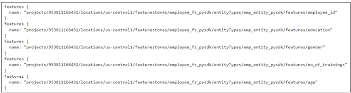
feature_selector=FeatureSelector(id_matcher=IdMatcher(ids=[“employee_id”,”education”,”gender”,”no_of_trainings”,”age”])),
)
)
print(resp_data)

The output will be stored in the resp_data variable and it is an iterator. Run the following lines of code to extract and parse the data from the iterator:
names_col=[]
for resp in resp_data:
if resp.header.feature_descriptors != “”:
for head in resp.header.feature_descriptors:
names_col.append(head.id)
try:
values=[]
for items in resp.entity_view.data:
if items.value.string_value !=””:values.append(items.value.string_value)
elif items.value.int64_value !=””:values.append(items.value.int64_value)
except:pass
print(“Feature Names”,names_col)
print(“Feature Values”,values)

The output of the cell is shown in Figure 9.21:

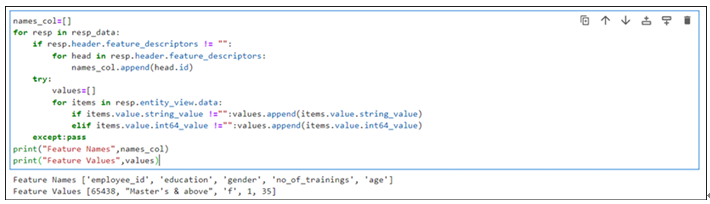
Figure 9.21: Data extracted from the feature store
Deleting resources
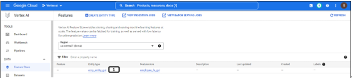
We have utilized cloud storage to store the data and delete the CSV file from the cloud storage manually. Feature store is a cost-incurring resource on GCP, ensure to delete them. Also, the feature store cannot be deleted from the web console or GUI, we need to delete it through programming. Run the below-mentioned lines of code to delete the feature store (both the feature stores were created using GUI and Python). Check if the landing page of the feature store after running the code to ensure it is deleted (the landing page should look like the Figure 9.4):
client_admin.delete_featurestore(
request=fs_s.DeleteFeaturestoreRequest(
name=client_admin.featurestore_path(Project_id, location, featurestore_name),
force=True,
)
).result()
featurestore_name=employee_fs_gui
client_admin.delete_featurestore(
request=fs_s.DeleteFeaturestoreRequest(
name=client_admin.featurestore_path(Project_id, location, featurestore_name),
force=True,
)
).result()

Best practices for feature store

Below listed are few of the best practices for using Feature store of Vertex AI:

1. Model features to multiple entities: Some features might be used in multiple entities (like clicks per product at user level). In this kind of scenarios, it is best to create a separate entity to group shared features.
2. Access control for multiple teams: Multiple teams like data scientists, ML researchers, Devops, and so on, may require access to the same feature store but with different level of permissions. Resource level IAM policies can be used to restrict the access to feature store or particular entity type.
3. Ingesting historical data (backfilling): It is recommended to stop online serving while ingesting the historical data to prevent any changes to the online store.
4. Cost optimization:
   1. Autoscaling: Instead of maintaining a high node count, autoscaling allows Vertex AI Feature Store to analyze traffic patterns and automatically modify the number of nodes up or down based on CPU consumption and also works better for cost optimization.
   1. Recommended to provide a startTime in the batchReadFeatureValues or exportFeatureValues request to optimize offline storage costs during batch serving and batch export.

Conclusion

In this chapter, we learned about the feature store of Vertex AI, and worked on the creation of the feature store, entity type, adding features, and ingesting feature values using web console and Python.

In the next chapter, we will start understanding explainable AI, and how explainable AI works on Vertex AI.

Questions

1. What are the different input sources from which data can be ingested into a feature store?
2. Can feature stores have multiple entity types?
3. What are the scenarios in which using a feature store brings value?

Step 8: Creation of entity type
Entity type will be created under the newly created feature store using the create_entity_type method. Run the below-mentioned code in a new cell to create the entity type. The output of the last line in the code provides the path of the entity type created. Check the feature store landing page, the newly created feature store, and the entity type will be displayed:
entity_creation = client_admin.create_entity_type(
fs_s.CreateEntityTypeRequest(
parent=client_admin.featurestore_path(Project_id, location, featurestore_name),
entity_type_id=Entity_name,
entity_type=entity_type.EntityType(
description=”employee entity”,
),
)
)
print(entity_creation.result())

Step 9: Creation of feature
Once the feature store and entity type are created, the feature needs to be created before ingesting the feature values. For each of the features, information on feature ID, type, and description is provided. Run the following-mentioned code in a new cell to add features:
client_admin.batch_create_features(
parent=client_admin.entity_type_path(Project_id, location, featurestore_name, Entity_name),
requests=[
fs_s.CreateFeatureRequest(
feature=feature.Feature(
value_type=feature.Feature.ValueType.INT64,
description=”employee id”,
),
feature_id=”employee_id”,
),
fs_s.CreateFeatureRequest(
feature=feature.Feature(
value_type=feature.Feature.ValueType.STRING,
description=”education”,
),
feature_id=”education”,
),
fs_s.CreateFeatureRequest(
feature=feature.Feature(
value_type=feature.Feature.ValueType.STRING,
description=”gender”,
),
feature_id=”gender”,
),
fs_s.CreateFeatureRequest(
feature=feature.Feature(
value_type=feature.Feature.ValueType.INT64,
description=”no_of_trainings”,
),
feature_id=”no_of_trainings”,
),
fs_s.CreateFeatureRequest(
feature=feature.Feature(
value_type=feature.Feature.ValueType.INT64,
description=”age”,
),
feature_id=”age”,
),
],
).result()

Once the features are created, they are displayed in the output of the cell as shown in Figure 9.19:

Figure 9.19: Addition of features to the feature store using Python

Step 10: Define the ingestion job
As seen in the web console, feature values can be ingested from cloud storage or BigQuery. We shall use the same CSV file which has been uploaded to the cloud storage. Importantly, we should also supply the timestamp information while ingesting the values. Timestamps can be provided in the code or there can be a separate column in the data that contains timestamp information. Timestamp information must be in google.protobuf.Timestamp format. Run the following code in a new cell to define the ingestion job:
seconds = int(datetime.datetime.now().timestamp())
timestamp_input = Timestamp(seconds=seconds)
ingest_data_csv = fs_s.ImportFeatureValuesRequest(
entity_type=client_admin.entity_type_path(
Project_id, location, featurestore_name, Entity_name
),
csv_source=io.CsvSource(
gcs_source=io.GcsSource(
uris=[
“gs://feature_store_input/employee_promotion_data_fs.csv”
]
)
),
entity_id_field=”employee_id”,
feature_specs=[
ImportFeatureValuesRequest.FeatureSpec(id=”employee_id”),
ImportFeatureValuesRequest.FeatureSpec(id=”education”),
ImportFeatureValuesRequest.FeatureSpec(id=”gender”),
ImportFeatureValuesRequest.FeatureSpec(id=”no_of_trainings”),
ImportFeatureValuesRequest.FeatureSpec(id=”age”),
],
feature_time=timestamp_input,
worker_count=1,
)

Note: If all feature values were generated at the same time, there is no need to have a timestamp column. Users can specify the timestamp as part of the ingestion request.
Step 11: Initiation of ingestion job
The ingestion job needs to be initiated after it is defined, run the following line of codes to begin the ingestion process:
ingest_data = client_admin.import_feature_values(ingest_data_csv)
ingest_data.result()

Once the ingestion is complete, it will provide information on the number of feature values ingested as shown in Figure 9.20:

Figure 9.20: Ingestion of feature values using Python

Step 6: Entity type created successfully

The entity type is created successfully as shown in Figure 9.8 under the selected feature store:

Figure 9.8: Entity type created and listed on the landing page

1. Click the newly created Entity type.

Step 7: Creation of features

Once the entity type is created, features need to be created before ingesting the values. Follow the steps mentioned in Figure 9.9 to create features:

Figure 9.9: Creation of features

1. Click ADD FEATURES.

A new side tab will pop out to enter the features as shown in Figure 9.10, follow the below steps to create the features:

Figure 9.10: Adding user input for feature creation

2. Enter the Feature name.
3. Enter the Value type stored in that feature.
4. Enter the Description for the feature.
5. Click Add Another Feature to add new features.
6. Click SAVE, once all the features are added.

Step 8: Features created successfully

Once the features are created successfully, they are displayed on the entity type page as shown in Figure 9.11:

Figure 9.11: Features listed under the entity type

1. Newly created features are displayed in tabular format.
2. Click on Ingest Values to add the feature values.

Step 9: Ingesting feature values

Follow the steps mentioned in Figure 9.12 to initiate the ingestion of feature values:

Figure 9.12: Importing data to features

1. Data can be ingested from cloud storage or BigQuery. Select Cloud Storage CSV file.
2. Select the CSV file from the cloud storage by clicking BROWSE.
3. Click CONTINUE and follow the steps mentioned in Figure 9.13:

After selecting the data source, we need to map the columns of the data source to the features. Follow the steps mentioned in the Figure 9.13 to map the features:

Figure 9.13: Mapping of columns to features

1. Add employee ID, since that is the column which is containing unique values.
2. Select to enter the Timestamp manually. If data contains the timestamp values, the same column can be used here.
3. Select the date and time.
4. Map the column names in the CSV file to the features.
5. Click INGEST to initiate the ingestion job.

Step 10: Ingestion job successful

Once the feature values are ingested successfully, the ingestion job status will be updated as shown in Figure 9.14:

Figure 9.14: Ingestion jobs of feature store

1. The ingestion job is completed successfully.

Step 11: Landing page of feature store after the creation of feature store, entity type, and features

The landing page of the feature store is shown in Figure 9.15, all the features under entity type and feature store are listed and displayed in the tabular format:

Figure 9.15: Landing page of feature store after the creation of features

1. Click the age feature. The window will navigate to the properties of the feature as shown in Figure 9.16:

Figure 9.16: Properties of feature

1. For all the features, Feature Properties consisting of basic information and statistics are displayed.
2. Metrics are populated if the monitoring feature is enabled for the feature store and for that particular feature.

These are the advantages of feature store:

• Extend features company-wide: Feature stores let you easily share features for training or serving. Different projects and use cases do not need feature re-engineering. Manage and deliver features from a central repository to preserve consistency throughout your business and prevent redundant efforts, especially for high-value features.

Vertex AI Feature Store lets people find and reuse features using search and filtering. View feature metadata to assess quality and usage. For instance, you may check feature coverage and feature value distribution.

• Serving at scale: Online forecasts require low-latency feature serving, which Vertex AI Feature Store manages. Vertex AI Feature Store automatically builds and expands low-latency data serving infrastructure. You create features but outsource providing them. Data scientists may create new features without worrying about deployment using this management.
• Reduce training-serving bias: Training-serving skew happens when your production feature data distribution differs from the one used to train your model. This skew causes disparities between a model’s training and production performance. Vertex AI Feature Store can handle training-serving bias with these examples:
  • Vertex AI Feature Store guarantees that feature values are ingested once and reused for training and serving. Without a feature store, training and serving features may use distinct code paths. Training and serving feature values may differ.
  • Vertex AI Feature Store offers previous data lookups for training. By collecting pre-prediction feature values, these lookups reduce data leakage.
• Identify drift: Vertex AI Feature Store detects drift in feature data distribution. Vertex AI Feature Store monitors feature value dispersion. Retrain models using impacted features as feature drift rises.
• Retention: The Vertex AI Feature Store preserves feature values for the allotted amount of time. This cap is determined by the feature values’ timestamp, not the date and time the values were imported. Values with timestamps that go beyond the limit are scheduled for deletion by Vertex AI Feature Store.

Disadvantages of feature store

A feature store has overhead, which can make data science more complicated, especially for smaller projects. A feature store may complicate matters if a business has numerous little data sets. Feature stores are ineffective when the data is so diverse that no standard modeling approach will assist. Reusing features created on separate data sources and metadata is tough. Additionally, a feature store might not be the ideal choice when the features are not time-dependent or when features are needed only for batch predictions.

Step 6: Creation of pipeline
Till now we have understood and executed certain components of the tfx pipeline (not all the components are needed for the pipeline construction). Let’s start constructing pipeline using example_gen, statistics_gen, schema_gen, transform, trainer and pusher components (Pusher component is used to push the trained model to a location, in this example trained model we will be pushed to the cloud storage):
• Define a function (_create_pipeline) to consisting of all the steps/components that needs to be included in the pipeline and returns the tfx pipeline. Run the below mentioned code in a new cell to define the pipeline function:
def _create_pipeline(pl_name, pipeline_root_folder, data_root,
module_file_transform, module_file_train, model_dir_save,
) -> tfx.dsl.Pipeline:
example_gen_csv = tfx.components.CsvExampleGen(input_base=data_root)
gen_statistics = tfx.components.StatisticsGen(examples=example_gen_csv.outputs[‘examples’])
gen_schema = tfx.components.SchemaGen(statistics=gen_statistics.outputs[‘statistics’])
transform_data = tfx.components.Transform(examples=example_gen_csv.outputs[‘examples’],schema=gen_schema.outputs[‘schema’],module_file=os.path.join(MODULE_FOLDER, TRANSFORM_MODULE_PATH))
model_trainer = tfx.components.Trainer(
module_file=module_file_train,
examples=example_gen_csv.outputs[‘examples’],
transform_graph=transform_data.outputs[‘transform_graph’],
schema=gen_schema.outputs[‘schema’],
train_args=tfx.proto.TrainArgs(num_steps=200),
eval_args=tfx.proto.EvalArgs(num_steps=10))
pusher = tfx.components.Pusher(
model=model_trainer.outputs[‘model’],
push_destination=tfx.proto.PushDestination(
filesystem=tfx.proto.PushDestination.Filesystem(
base_directory=model_dir_save)))
return tfx.dsl.Pipeline(
pipeline_name=pl_name,
pipeline_root=pipeline_root_folder,
components=[example_gen_csv,gen_statistics,gen_schema,transform_data,model_trainer,pusher])

Step 8: Defining a runner
As mentioned in the theory section, TFX is portable across environments and orchestration frameworks. TFX supports Airflow, Beam, and Kubeflow. It also provides flexibility for the developers to add their own orchestrators. Orchestrators must inherit TfxRunner. TFX orchestrators schedule pipeline components based on DAG dependencies using the logical pipeline object, which comprises pipeline args, components, and DAG. In our example we will be using Vertex Pipelines together with the Kubeflow V2 dag runner. In the code, we create runner using Kubeflow V2 dag and run it by passing all the pipeline parameters.
Run the following mentioned codes to define the runner:
trainer_file=”trainer.py”
file_transform=os.path.join(MODULE_FOLDER, TRANSFORM_MODULE_PATH)
file_train=os.path.join(MODULE_FOLDER, trainer_file)
pl_def_file = NAME_PIPELINE + ‘.json’
pl_runner = tfx.orchestration.experimental.KubeflowV2DagRunner(
config=tfx.orchestration.experimental.KubeflowV2DagRunnerConfig(),
output_filename=pl_def_file)
_ = pl_runner.run(
_create_pipeline(
pl_name=NAME_PIPELINE,
pipeline_root_folder=ROOT_PIPELINE,
data_root=INPUT_DATA_DIR,
module_file_transform=file_transform,
module_file_train=file_train,
model_dir_save=OUTPUT_MODEL_DIR))

Step 9: Pipeline execution
As the last step we need to execute the pipeline. Run the following mentioned codes in a new cell to start the pipeline execution:
import google.cloud
google.cloud.aiplatform.init(project=PROJECT_ID, location=”us-central1”)
job=google.cloud.aiplatform.pipeline_jobs.PipelineJob(template_path=pl_def_file,
display_name=NAME_PIPELINE)
job.run(sync=False)

Once the pipeline starts, users will be provided the link to check the status as shown in Figure 8.13:

Figure 8.13: Pipeline link

1. Click on the link to check the status of the pipeline as shown in the following screenshot:

Figure 8.14: Pipeline executed successfully
Pipeline will take a few mins to complete the training and push the trained model to the cloud storage. If the pipeline is constructed using tfx or Kubeflow, the user interface of the pipeline in GCP will remain same as shown in Figure 8.14. Spend some time to understand each of the components and its artifacts in detail as described in the previous chapter.

Transform:
We will create file_transform.py which will contain information about the data labels and feature engineering steps:
• Run the following mentioned code in new cells to declare variable containing file name:
TRANSFORM_MODULE_PATH = ‘file_transform.py’

• Run the following mentioned codes in a new cell to create file_transform.py file. Preprocessing (preprocessing_fn) function is where the actual alteration of the dataset occurs. It receives and returns a tensor dictionary, where tensor refers to a Tensor or SparseTensor. In our example, we are not applying any transformations, code is just mapping to the output dictionary. (%%writefile command will create the .py file with the following code in it.):
%%writefile {TRANSFORM_MODULE_PATH}
import tensorflow as tf
import tensorflow_transform as tft
NAMES = [‘AF3’,’F7’,’F3’,’FC5’,’T7’,’P7’,’O1’,’O2’,’P8’,’T8’,’FC6’,’F4’,’F8’,’AF4’]
LABEL = ‘eyeDetection’
def preprocessing_fn(raw_inputs):
processed_data = dict()
for items in NAMES:
processed_data[items]=raw_inputs[items]
processed_data[LABEL] = raw_inputs[LABEL]
return processed_data

3. Files needs to copy into GCS bucket, run the following line of code to copy it:
   !gsutil cp file_transform.py {MODULE_FOLDER}/
4. Run the following mentioned lines of codes in a new cell to configure transform component. Transform component is taking inputs from the example_gen and schema_gen:
   transform_data = tfx.components.Transform(
   examples=example_gen_csv.outputs[‘examples’],schema=gen_schema.outputs[‘schema’],
   module_file=os.path.join(MODULE_FOLDER, TRANSFORM_MODULE_PATH))
   context_in.run(transform_data, enable_cache=False)

Output of the transform component is as shown in Figure 8.10. Transform graph is one of the artifacts generated by the transform component and it will be used for the trainer module.

Figure 8.10: Output of transform component
Run the following mentioned codes to check few records of the transformed data (This code will not be needed during the pipeline construction):
train_sam = os.path.join(transform_data.outputs[‘transformed_examples’].get()[0].uri,’Split-train’)
filenames_tfr = [os.path.join(train_sam, name) for name in os.listdir(train_sam)]
dataset = tf.data.TFRecordDataset(filenames_tfr, compression_type=’GZIP’)

for record in dataset.take(1):
sample = tf.train.Example()
sample.ParseFromString(record.numpy())
print(sample)

Output of 1 record will be as shown in Figure 8.11:

Figure 8.11: Transformed data example
Trainer:
The Trainer component is in charge of preparing the input data and training the model. It requires the ExampleGen examples, the transform, and the training code. TensorFlow Estimators, Keras models, or custom training loops can be used in the training code. When compared to other components, trainer requires more modifications in the code:
• Run the following mentioned code in the new cell, it will generate trainer.py file (Complete code is available in the repository). Trainer.py (training code) file will be the input for the trainer module. Trainer component generates two artifacts model (trained model itself) and modelrun which can be used for storing logs, this can be seen in Figure 8.12. The Trainer.py file contains four functions; high level description of those functions is:
o run_fn will be entry point to execute the training process
o _input_fn generates features and labels for training
o _get_serve_tf_examples_fn returns a function that parses a serialized tf.example
o _make_keras_model creates and returns the model for classification
%%writefile trainer.py
from typing import List
from absl import logging
import tensorflow as tf
import tensorflow_transform as tft
from tensorflow import keras
from tensorflow_transform.tf_metadata import schema_utils
from tfx import v1 as tfx
from tfx_bsl.public import tfxio
from tensorflow_metadata.proto.v0 import schema_pb2

COL_NAMES=[‘AF3’,’F7’,’F3’,’FC5’,’T7’,’P7’,’O1’,’O2’,’P8’,’T8’,’FC6’,’F4’,’F8’,’AF4’]
LABEL=”eyeDetection”
BATCH_SIZE_TRAIN = 40
BATCH_SIZE_EVAL = 20
def _input_fn(files,accessor,transform_output,size) -> tf.data.Dataset:
Creates datasets and apply transformations on them and return.
Refer the repository for code block of the function
return dataset.map(apply_transform_fn).repeat()
def _get_serve_tf_examples_fn(model, transform_output):
To parse the serialized examples and return.
Refer the repository for code block of the function
return serve_tf_examples_fn
def _make_keras_model() -> tf.keras.Model:
Create model with layers, loss functions to be used and return.
Refer the repository for code block of the function
return model_classification

def run_fn(fn_args: tfx.components.FnArgs):
tf_transform = tft.TFTransformOutput(fn_args.transform_output)
train_samples = _input_fn(_args.train_files, _args.data_accessor, tf_transform, =BATCH_SIZE_TRAIN)
eval_samples = _input_fn(_args.eval_files, _args.data_accessor, tf_transform, =BATCH_SIZE_EVAL)
model_classification = _make_keras_model()
model_classification.fit(
train_samples,
steps_per_epoch=fn_args.train_steps,
validation_data=eval_samples,
validation_steps=fn_args.eval_steps)
sign = {
“serving_default”: _get_serve_tf_examples_fn(model_classification, tf_transform),
}
model_classification.save(fn_args.serving_model_dir, save_format=’tf’,signatures=sign)

1. Run the following code to copy the trainer.py to GCS storage:
   !gsutil cp trainer.py {MODULE_FOLDER}/
2. Run the following code to initiate the trainer component. trainer_file=”trainer.py”:
   trainer_file_path=os.path.join(MODULE_FOLDER, trainer_file)
   model_trainer = tfx.components.Trainer(
   examples=example_gen_csv.outputs[“examples”],
   transform_graph=transform_data.outputs[“transform_graph”],
   train_args=tfx.proto.TrainArgs(num_steps=200),
   eval_args=tfx.proto.EvalArgs(num_steps=10),
   module_file=trainer_file_path,
   )
   context_in.run(model_trainer, enable_cache=False)

The output of the trainer component is as shown in the following figure:

Figure 8.12: Output of the trainer component